Black and White Printing with Capture One Pro webinar resources and print offer

BLOG
Every Journey Needs a Journal
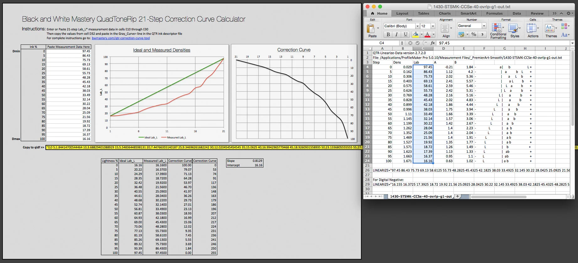
I don't mean for this to become a site dedicated to printing with QuadToneRIP, and I have a few new exciting things waiting in the wings that will be coming out in the next few months. In the mean time, here is a little tool I put together for automatically creating a QTR correction curve based on any 21-step measurement file, and outputs a set of input and output points that can be pasted into the QTR ink descriptor file. This takes the place of the option to embedded a Photoshop .acv curve in the gray_curve= line and eliminates the problem of clobbering your profile if you move or edit the .acv file.
Anyone who has made their own QTR profiles has probably incountered the annoying "Lab values not in order" error when trying to linearize their profile. While this tool might not solve that problem completely, it should produe a profile that will print with a fairly straight-line density increase that should get you through the final linearization steps without any additional problems.
I have not tested this for creating a correction curve for printing inkjet negatives for alternative processes, but it should would for that as well—at least in theory...
The instructions and screenshots below show the steps for aMac, but the process is nearly identical for the Windows QTRgui (or when working with the ink descriptor file in a plain text editor on Windows).
The resulting profile should print nearly linear and can be fine tuned with the standard linearization process.
The next few screenshots are of the ink graphs from a custom six-shade carbon/selenium blend I made for an upcoming show in August. I intentionally created the raw profile to print much darker and blocked up than I would have normally created it to demonsrate how close the correction curve can get to a QTR linearized profile. There were no reverals in the initial curve so the standard linearization would have worked. Similar to the new Linearize-Quad app Roy Harrington recently released, this tool effectively allows for a two-step linearization process. It might not be right for every situation, but is good to have in the tool box so you can get through profiling and get to printing faster.
I did a series of controlled tests this morning comparing measurements made from profiles using the standard QTR linearization method to those using the correction curve tool I created. I tested 4 variations of a new custom 6- ink profile using a mixture of Cone Carbon mixed with Cone Selenium shades 2-6 and STS Matte Black as a Shade 1. The same 21x4 measurement file was used to create a QTR linearization and Correction Curve for each of the different variations of the profile to ensure that a errors in the readings were not the cause of any irregularities between the two.
Most people use a 21 step (5% step) target for measuring and linearizing their QuadToneRIP profiles. Using the 21x4-random target is a step better, and I described this process in my post last year with instructions for using i1 Profiler to measure the linearization targets. While the 21-step target does a good-enough job with a 3 partition profile, sometimes a 51-step (2% K) target can show you where little bumps might be hiding between those 5% steps.
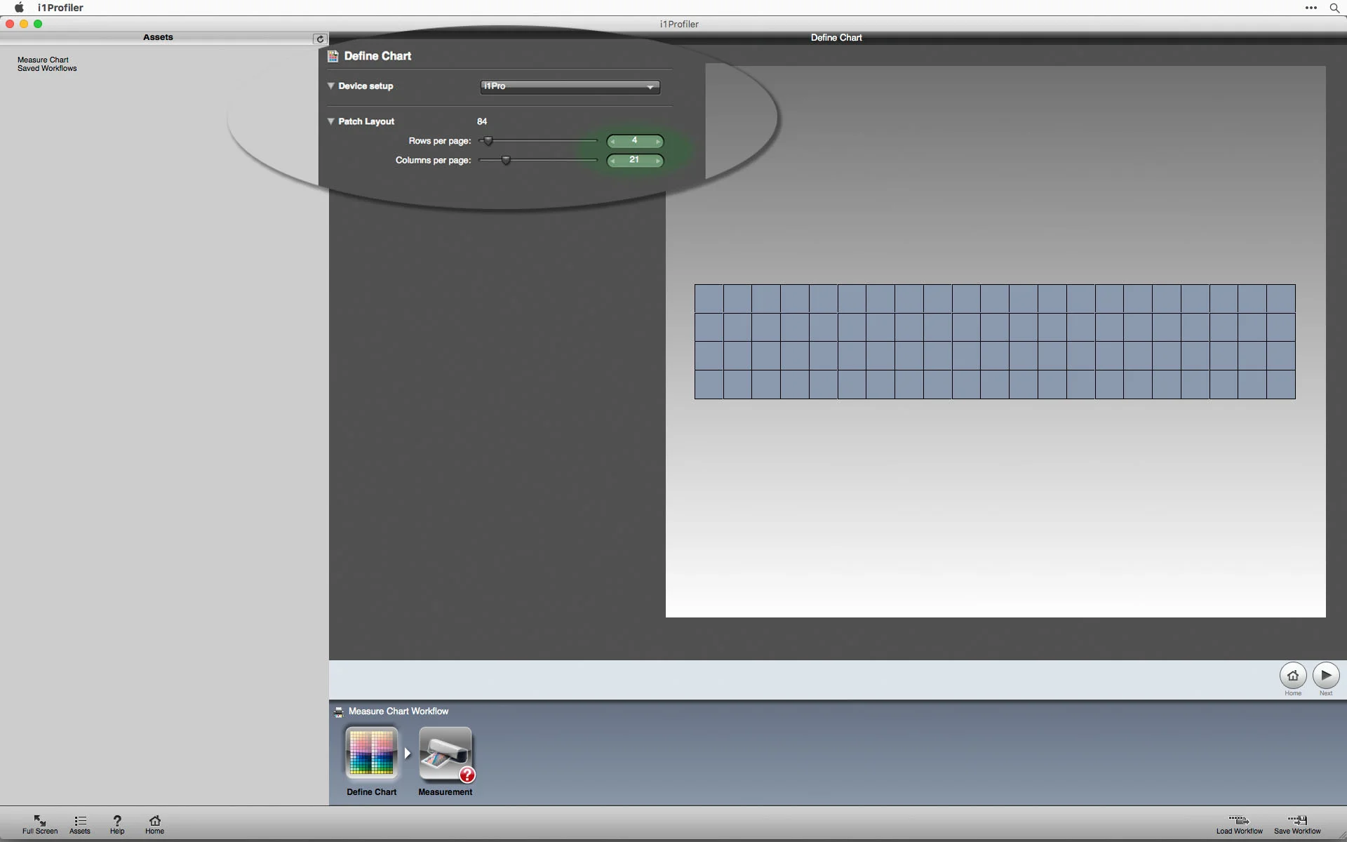
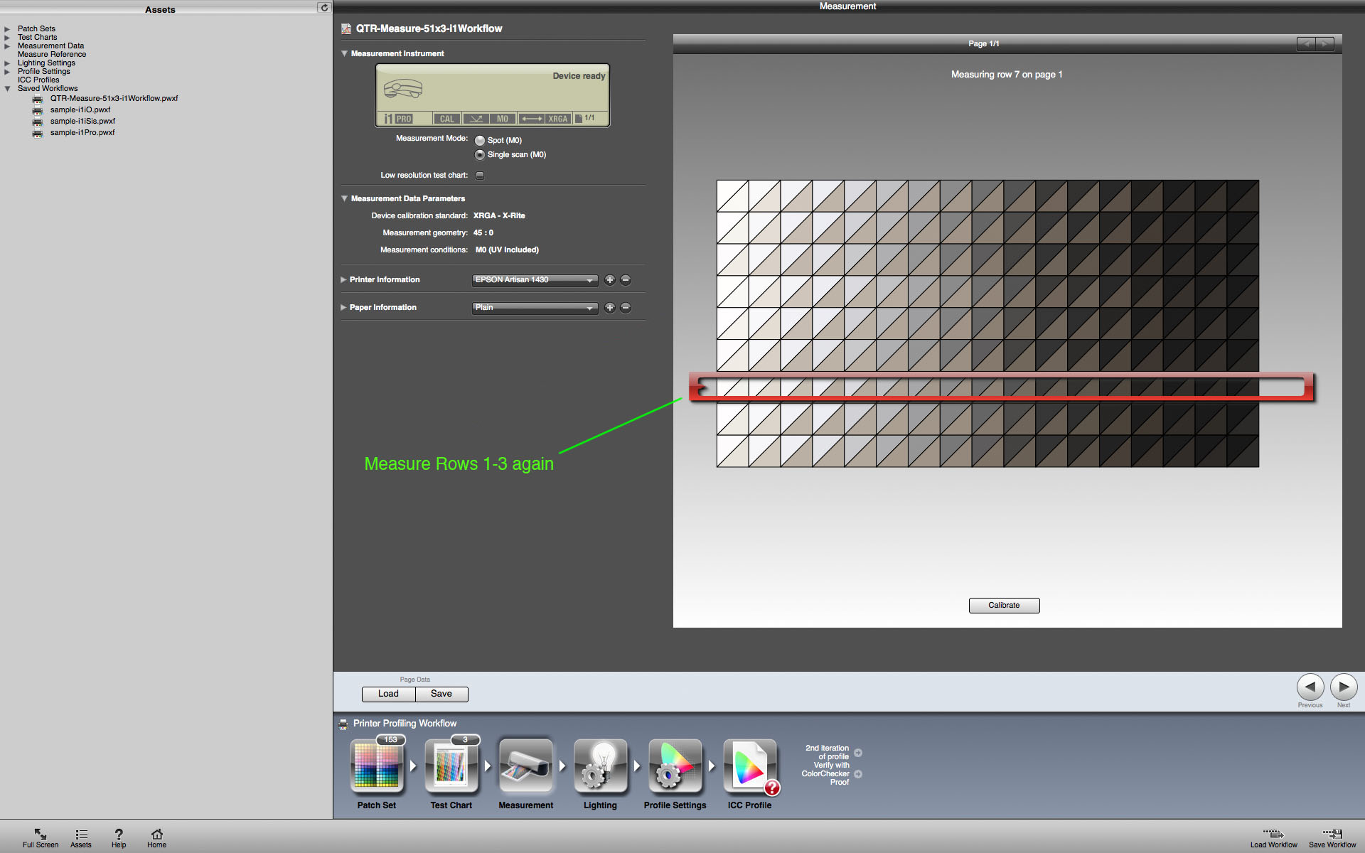
Measure a single patch a few times and you will see that it is usually off each time by a small percentage. Smaller steps will show more information, but can also show bumps in the curve where they might not actually exist. Those measurement errors need to be averaged out to determine if the problem is the actual ink distribution or inconsistencies in how the light reflects off the paper surface as the measuring device moves over each patch. After measuring thousands of patches over the last few years, I have settled on measuring each 51-step target 3 times. A 51x4 might be more accurate, but 9 passes seems to be about the limit of my patience… To make these averaging measurements easier, I have updated the 51-step 2% target included with QuadToneRIP so that it will work with i1 Profiler and the i1 Pro photospectrometer. The workflow allows you to measure the same target three times (measure row 1-3 once, and then go back and measure row 1-3 again when the on-screen instructions indicate measuring row 4-6, and measure it again when the instructions call for rows 7-9).
These instructions and screenshots were created on a Mac, but they are applicable to i1 Profiler for Windows. You will need to download the i1 Profiler from this Dropbox Link.
Print the 51-step target that is included in the downloaded zipfile from the QTRgui on windows or from PrintTool on Mac OSX and make sure to disable color managment. The larger format target that makes reading in strip mode requires you to print it in portrait orientation.
I suggest you create a folder on your desktop for the workflow and any saved measurement files. The default directory or folder for these files is buried in the Application Support folders on the Mac and in the Application Data (which is a hidden folder that can be revealed in the Tools>Folder Options Menu) in the Documents and Settings folder on Windows.
Mac:
Macintosh HD/Library/Application Support/X-Rite/i1Profiler/ColorSpaceRGB/PrinterProfileWorkflows
Windows:
C:\Documents and Settings\All Users\Application Data\X-Rite\i1Profiler\ColorSpaceRGB\PrinterProfileWorkflows
Drag workflow to this folder on Windows
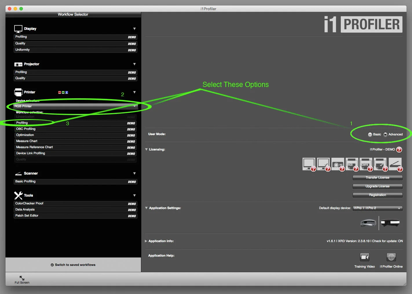
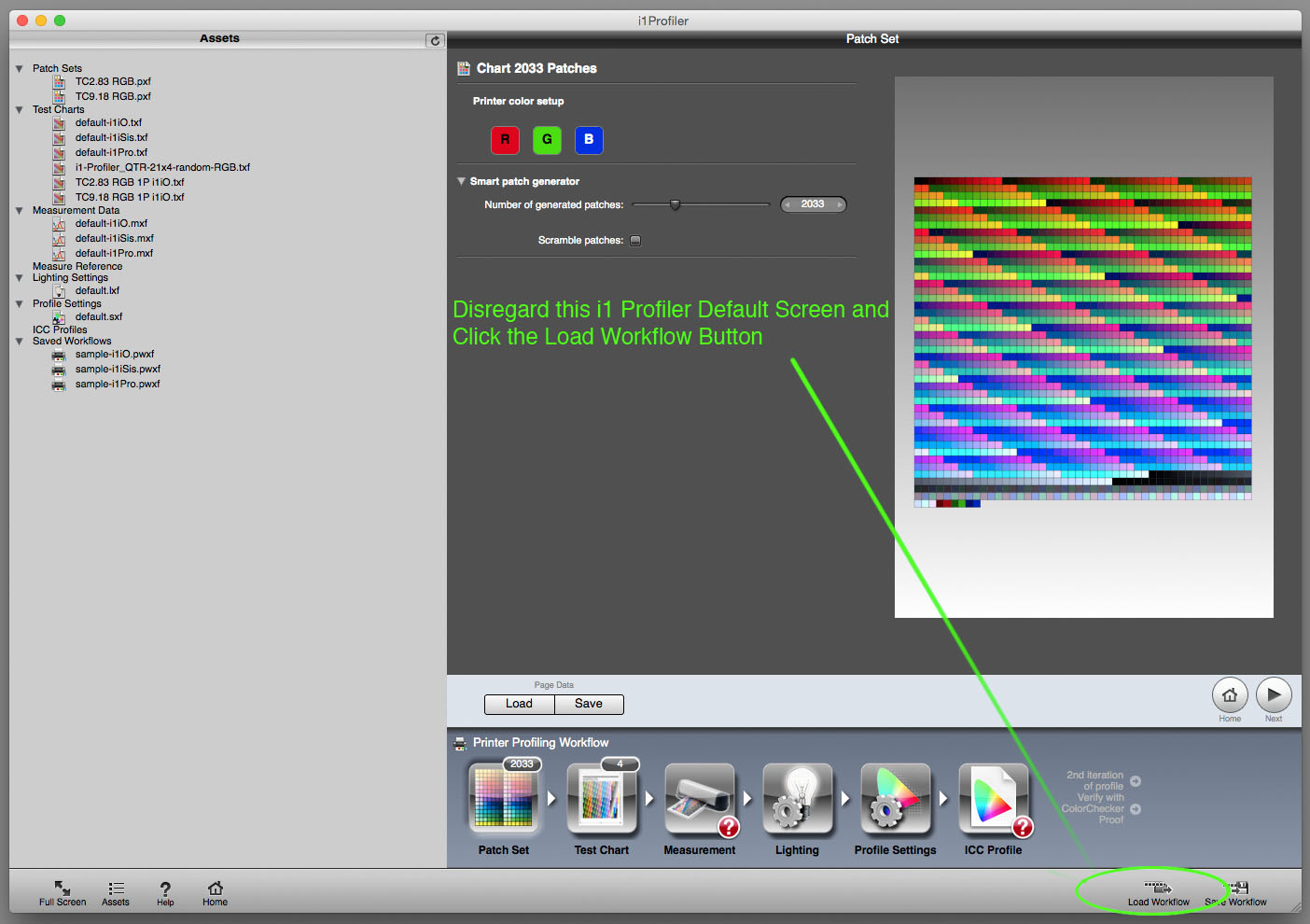
Launch the i1 Profiler Application and make sure you are in Advanced user mode. - Click either RGB or CMYK Printer - Click Profiling (this just gives you access to the next screen where you are able to load the saved workflow) - Alternatively, you can simply click "go to saved workflows" in the lower left portion of the screen.
To measure the chart three times:
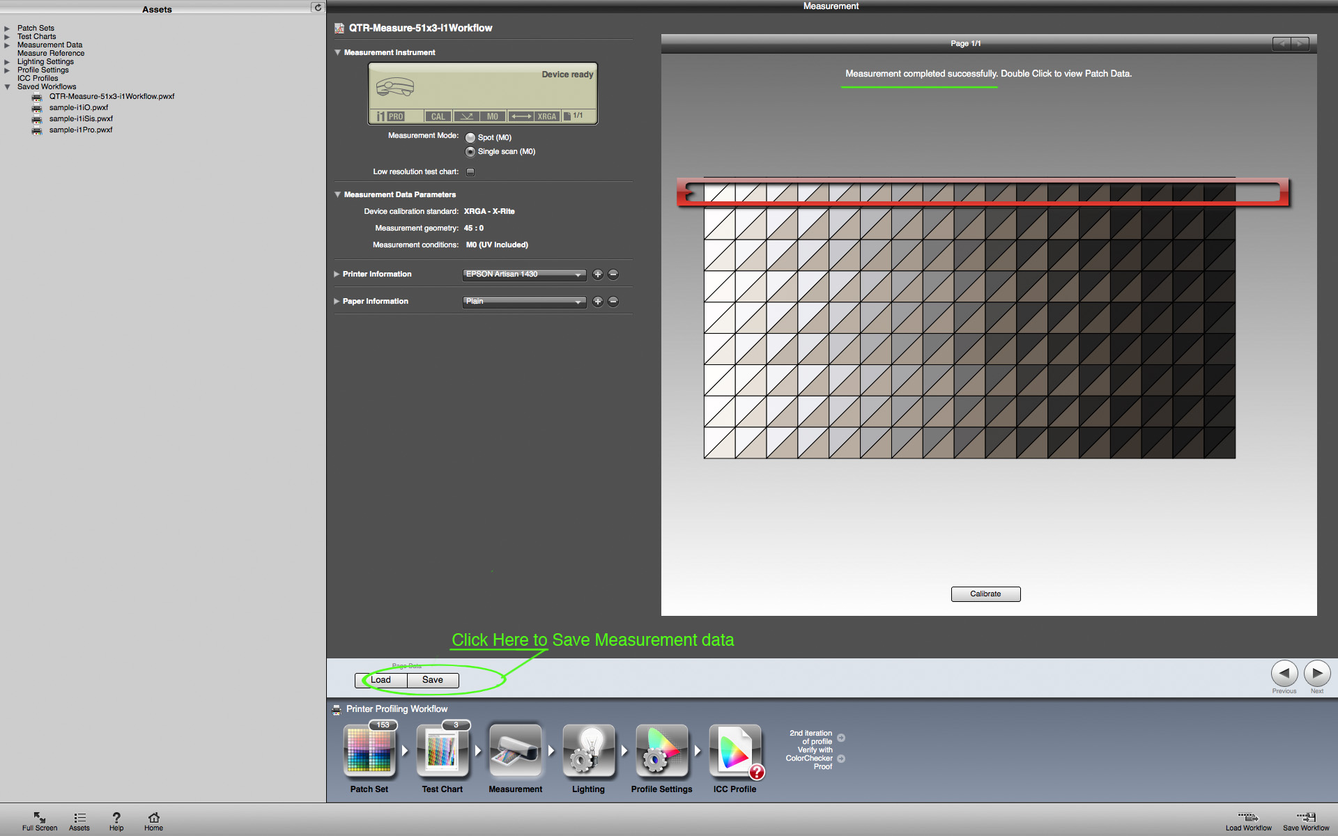
Saving the data in the correct format is essential for the automatic averaging and graphing template to recognize the correct data fields. This is also the correct data format for uploading your measurement file for my QTR Quad file relinearization service.
Create a relevant file name for the paper or the QTR profile/curves used to print the target. I generally suggest using the same name as the QTR or Piezography Profile being measured.
See the screenshot that illustrates the data fields to check.
When you click ok to accept it will save the file name you chose followed by “M0” ex: PaperName-ProfileNameM0 Open the file in a text editor to make sure it looks like the illustration below.
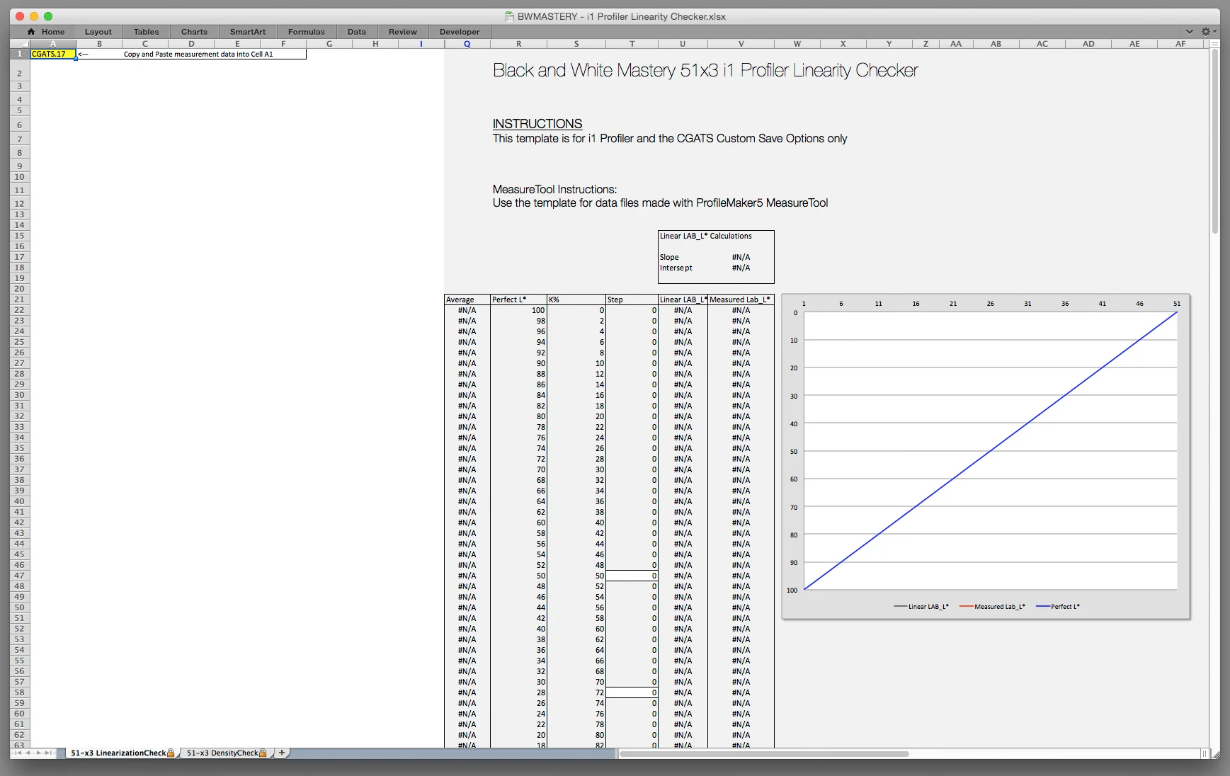
What good is measurement data if you can’t view it? Along with the workflow, I have added an Excel spreadsheet template that does an automatic lookup of the luminosity measurements and then averages and graphs them. The second sheet uses a different lookup to calculate Density from the recorded XYZ_Y measurements.
During a recent private Photoshop lesson with a student, we were attempting to address a problem with what what me be seen as “flare” around highlight areas that bleed into the mid-tones, giving it a mushy or muddy feeling. I introduced him to a type of detail enhancement that is often used for color images, but that I've adapted for increasing the detail of flatbed scans of prints being used in two differnt book projects I’m currently working on.
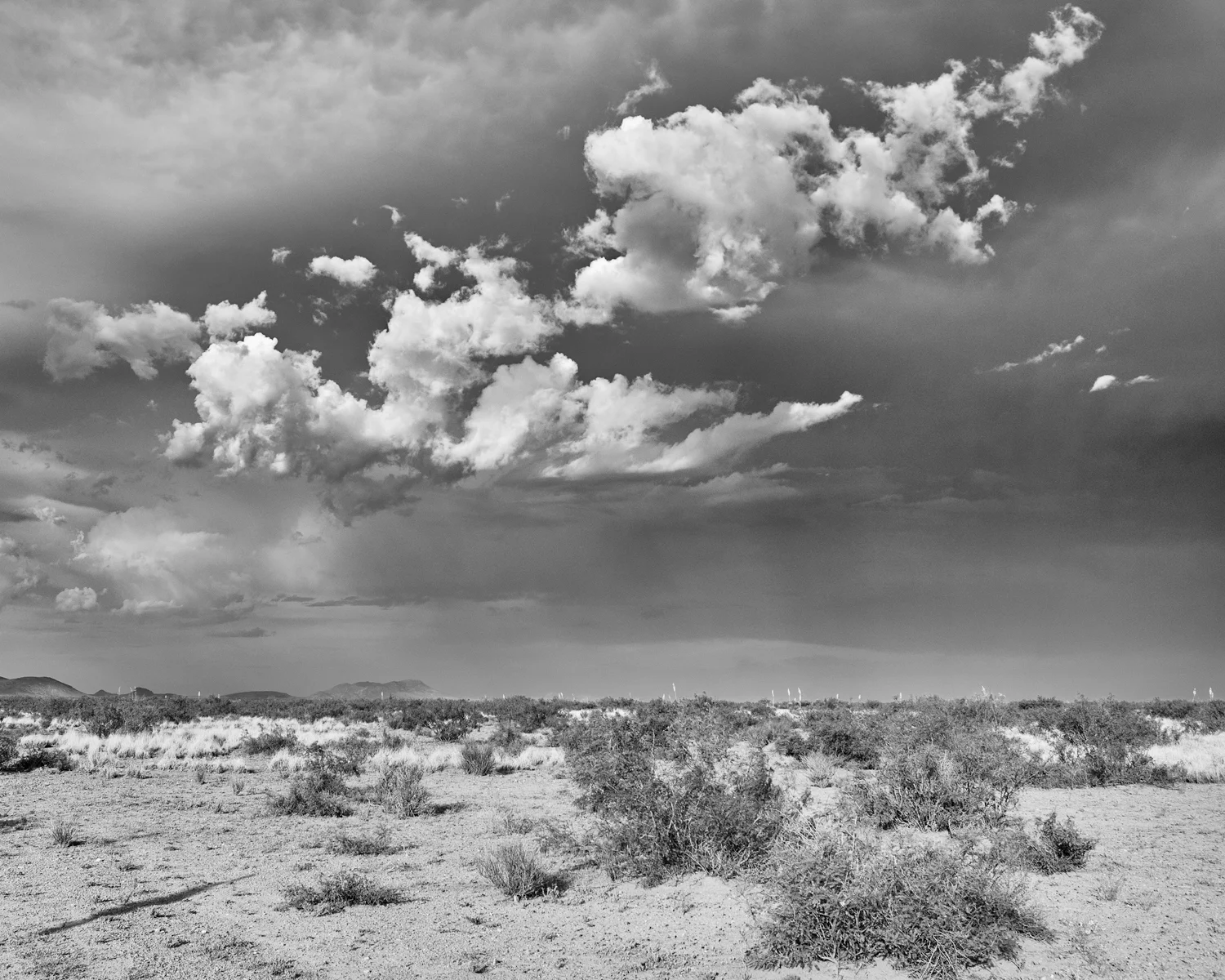
I am using the same image from the previous post comparing Capture 1 Pro 8 and Adobe Camera Raw to illustrate these steps. Fine details, like those in this picture, run the risk of quickly degrading if not carefully sharpened and masked, and the techniques shown here can be used to temper the sharpening or fine detail enhancements without blowing out detail, which can happen with other sharpening methods.
As a bonus I am making this photograph available as a part of a special discounted print offer on images used to illustrate select posts on this site. Read more about this offer at the end of this post or click here now.
Original Capture 1 Export. The mid-tones have a slightly blurred or flared look around the highlight areas. This first part of this workflows will remove the flare, and the second part will sharpen the mid-tone separation and fine detail.
You can see the problem in this first screen shot. The areas around the highlights look like they are flared so we can deal with that, and at the same time, increase some of the fine detail separation through out the who image.
The following series of steps are illustrated in the gallery of screenshots below.
Select Unsharp Mask from the Filter>Sharpen menu.
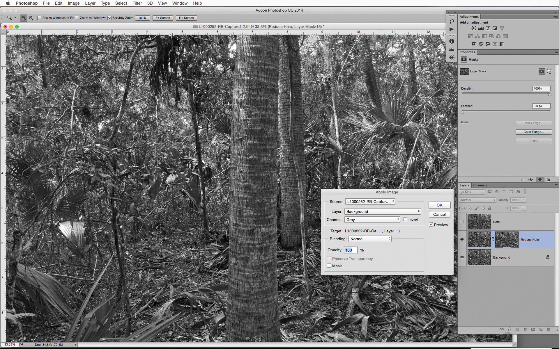
With the layer mask active, navigate to Apply Image in the Image menu.
Select background as the source and set the blend mode to Normal, and then click OK to accept. This will create a luminosity mask and make the "reduce halo" effect proportional to the tones in the image.
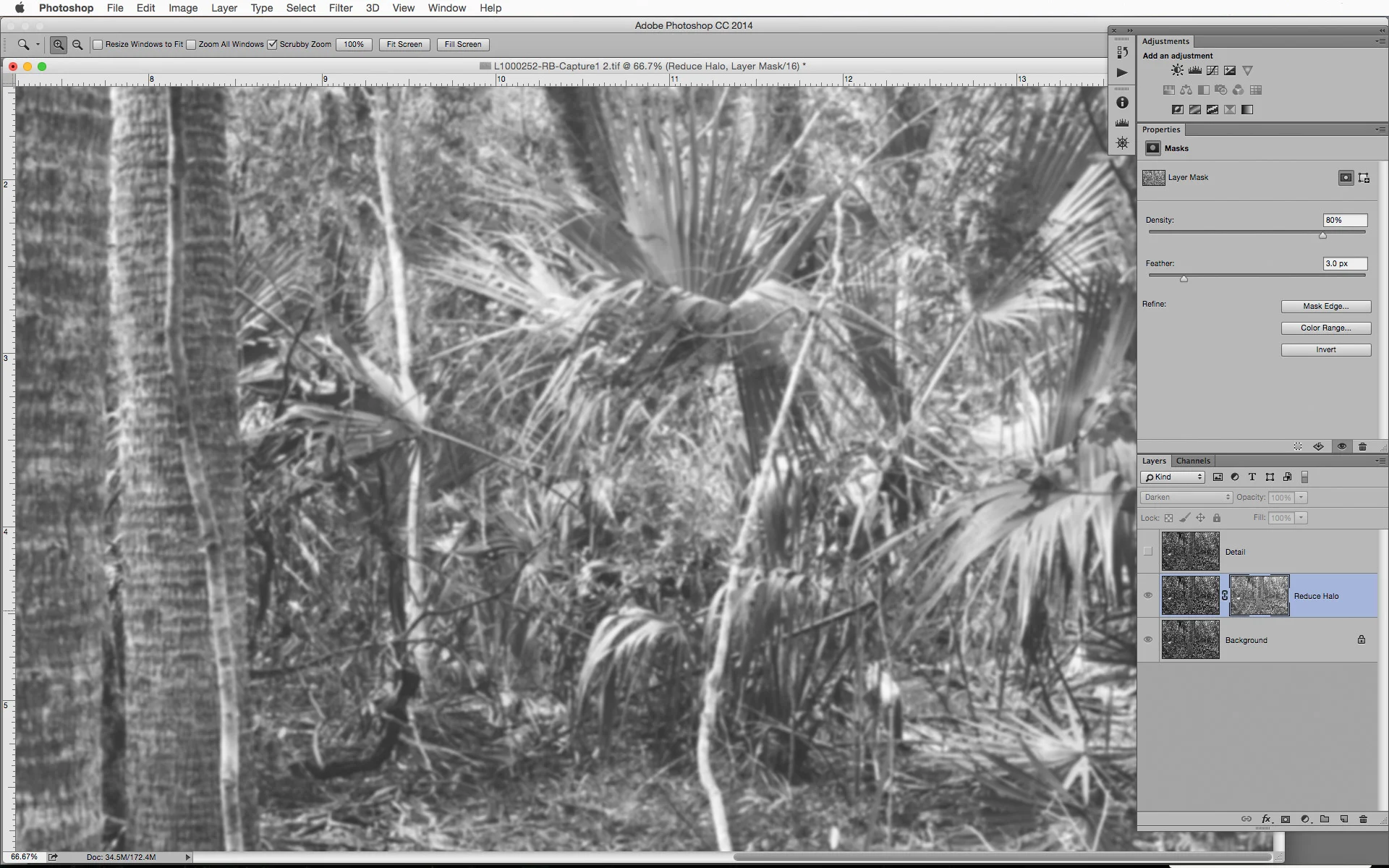
This effect can be further controlled in the Masks Panel by setting the feathering to a value between 2-5 pixels.
The range of tones affected can be controlled by applying a curves adjustment to the mask.
To do this, make the mask active and press option/alt while clicking in the mask icon, and then hit cmnd/cntrl+m to bring up the curves adjustment, and darken the shadow portion of the curve and lighten the highlights. It is important to note that once the curve is applied, it cannot be readjusted.
You can lower the density and readjust the feathering of the mask in the Masks Panel or lower the opacity of the layer to achieve the desired effect.
After making these adjustments to the mask, the original sharpening effect becomes very subtle, but helps enhance the mid-tone contrast so you are not increasing the appearance of any halos when making other lightening adjustments later in the editing process.
This short workflow and following series of steps is very similar to the "reduce halo" steps, but targets a different range of tones and uses slightly different settings. The screenshots at the end illustrate the different settings and what you masks and results should look like
Make the “Detail” layer active, and select unsharp mask from the Filer>Sharpen menu.
With the layer mask active, navigate to Apply Image in the Image menu.
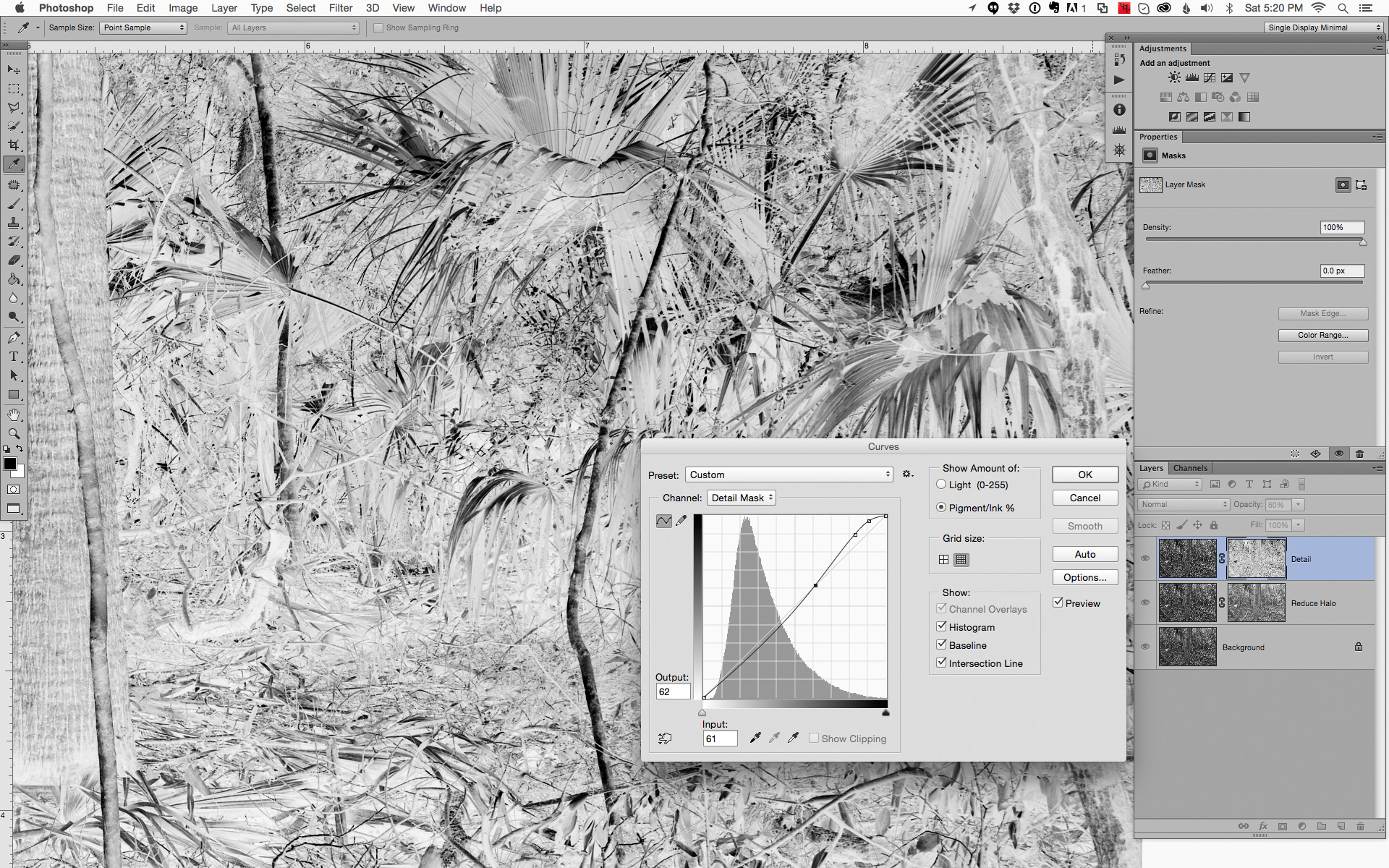
It can also be controlled by applying a curves adjustment to the mask.
To do this, make the mask active and press option/alt while clicking in the mask icon and then hit cmnd/cntrl+m to bring up the curves adjustment and darken the shadow portion of the curve and lighten the highlights. This is like applying an adjustment to an Alpha Channel and it is important to note that once the curve is applied, it is a destructive edit to the mask and cannot be reversed or undone further in the process.
Now go back to the layer opacity and change it to a value between 50%-70%, which should be sufficient in boosting the mid-tone separation and fine detail, without overdoing the effect.
With these adjustments made, you can proceed with any burning and dodging adjustments, with curves adjustment layers placed above the detail enhancement layers. With the added detail and separation created in these previous steps, additional contrast (if desired) will require less dramatic curves adjustments.
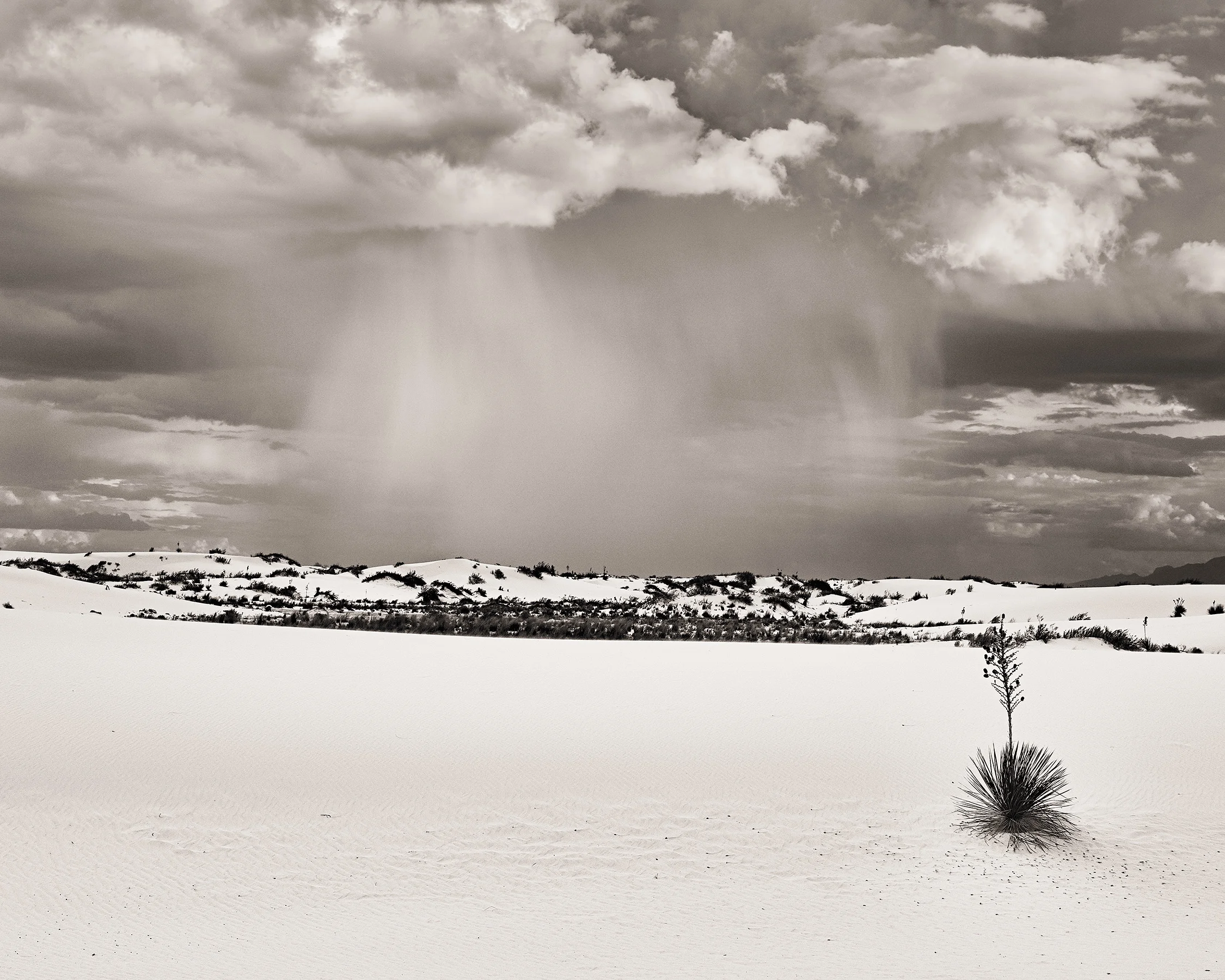
— 5.5"x9" signed and un-numbered print on 8.5"x11" paper
—12"x20" limited to an edition of 15 signed and numbered prints
Printed on Museo Portfolio Rag with a custom six gray ink blend of Jon Cone Piezography Carbon inks and STS Matte Black for additional density using my unique QuadToneRip profiling process.
I started to write about comparing Lightroom and Photoshop last year, but that turned into this post. I have been using Capture 1 Pro 7, and now version 8, as my default raw editor for exporting tiffs to Photoshop for final editing and output for the past year+ and haven't looked back. Until now... Adobe recently updated the Adobe Camera Raw processing engine and it is now included with the new Lightroom CC, and I was asked about testing how the Leica M Monochrome would benefit from Capture 1 compared to Lightroom CC or Adobe Camera Raw 9. Honestly, the differences between C1 and the new ACR are still astounding.
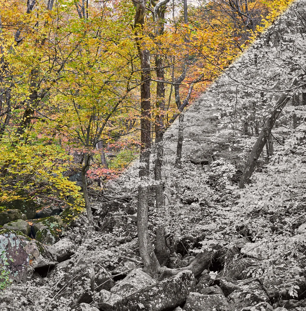
Adobe Camera Raw on left and Capture 1 Pro 8 on right at 100% pixel view
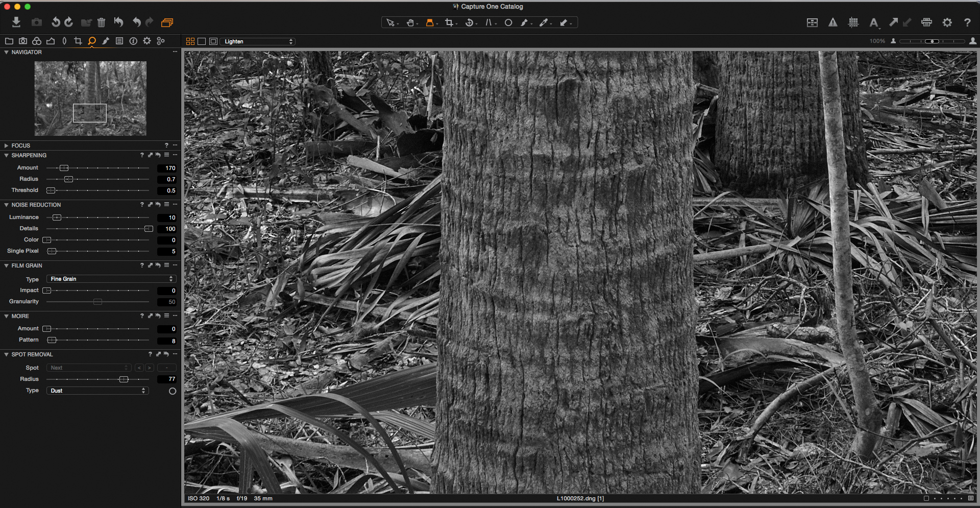
The above screenshot may make this blatantly obvious, but I will point out some areas where some subtle details benefit from the Capture 1 engine. There is something about the rendering of fine details and midtone separation that is so much better in C1, and it takes much less sharpening and clarity enhancement to achieve a perfectly sharp and smooth image. I would even say that it is sometime TOO much sharpness, and there is very little final sharpening that needs to be done in Photoshop.
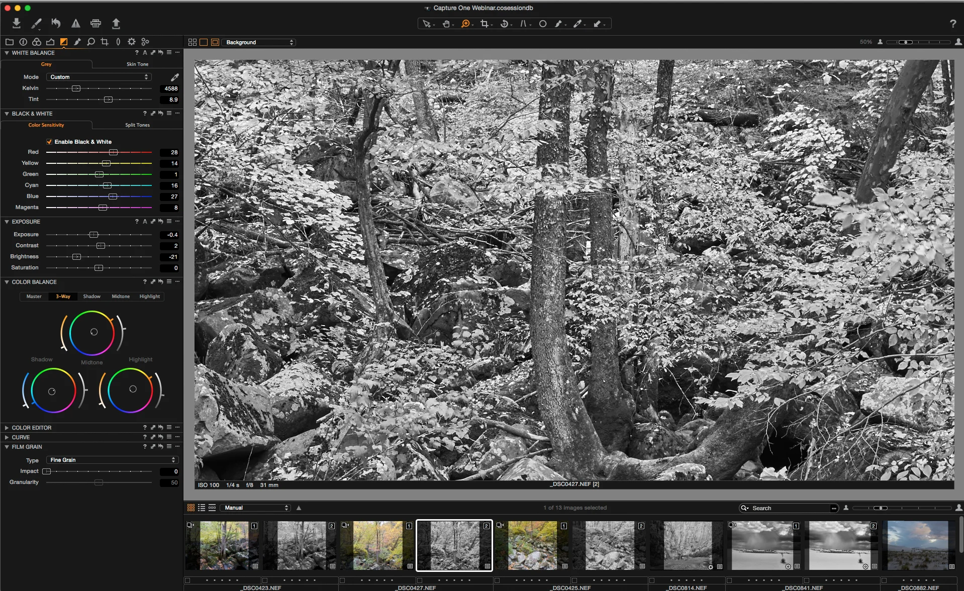
Here are some other screen shots with the detail and sharpening settings in both Capture 1 and Adobe Camera Raw. My personal sharpening settings are generally lower than the Capture 1 defaults, with only a small amount of Clarity and Structure in the detail settings. To arrive at comparable looking image in ACR, the clarity is cranked up to 64, and the sharpening and detail is much higher than the default of 25.
The benefits of Capture 1 are not all about sharpness and fine detail. The ability to select processing curve options allows you to create an initial tonal range that is tailored to the type of image and desired final outcome. Adobe Camera Raw has one default curve and all global tonal edits are done though the settings for exposure, contrast, highlights, etc.
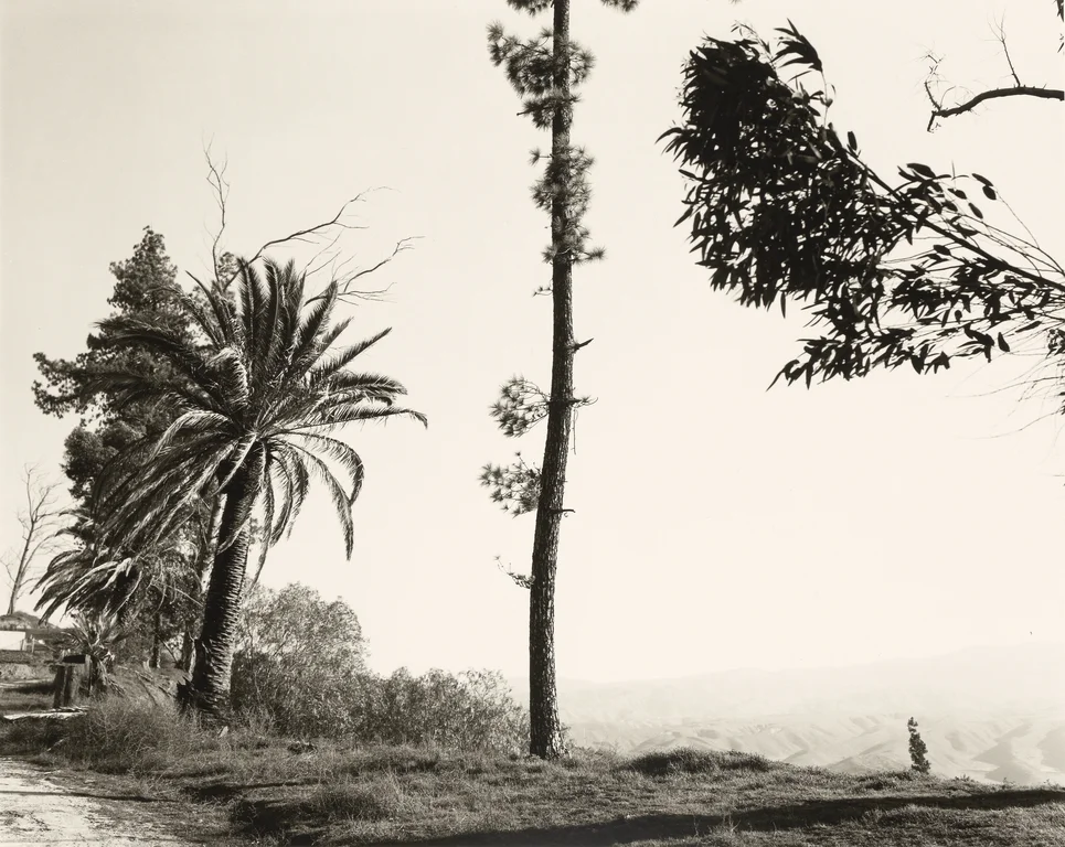
Washington Oaks, Florida 2013
Final edited version with warm-toned ink simulation
This was made during a private Digital Black and White Crash Course workshop near Daytona Beach, Florida with the student's Leica M Monochrome camera. The challenge was to see how much of the fine detail could be retained in the harsh lighting conditions, while still being able to make a coherent picture from the extremely dense and chaotic scene.
Be sure to read the next post, also working with the same image, to learn how to further enhance the detail from your photographs with some additional Photoshop Unsharp Mask techniques. Read to the end for a new special offer on photographs from select blog posts.
Please consider contributing a few dollars to enable me to continue to test new inks and papers and to develop free tools to help you take your work to the next level
(and not cluttering the site with annoying ads...)